Multivariate time series analysis: copper production forecasting
- Angel Aponte

- Mar 8, 2023
- 2 min read
Updated: Apr 7, 2023
Forecasting is the process of making predictions based on past and present data. Later these can be compared (resolved) against what happens. Forecasting might refer to specific formal statistical methods employing Time Series, Cross-Sectional or Longitudinal data, or to less formal judgmental methods or the process of prediction and resolution itself.

In this post, I present UNIVARIATE and MULTIVARIATE Time Series Machine Learning workflows. R language was used to perform the UNIVARIATE analysis. The MULTIVARIATE case was implemented in KNIME Analytics Platform, using an H2O.ai Linear Regression Learner and PARAMETER OPTIMIZATION. Data used in the following examples were gathered from the Chilean Copper Company CoChilCo official site.

In the UNIVARIATE case, to take into account the data autocorrelation and its highly-no-linearity, an Autoregressive NN Learner (ARNNL) was trained. Then five years forecast was performed. The figure above depicts the results of the UNIVARIATE Machine Learning modeling and forecasted Time Series. These results could be improved, by fine-tuning the ARNNL hyper-parameters. This task is always the most challenging-difficult-time-consuming stage of the entire training-test Machine Learning process.
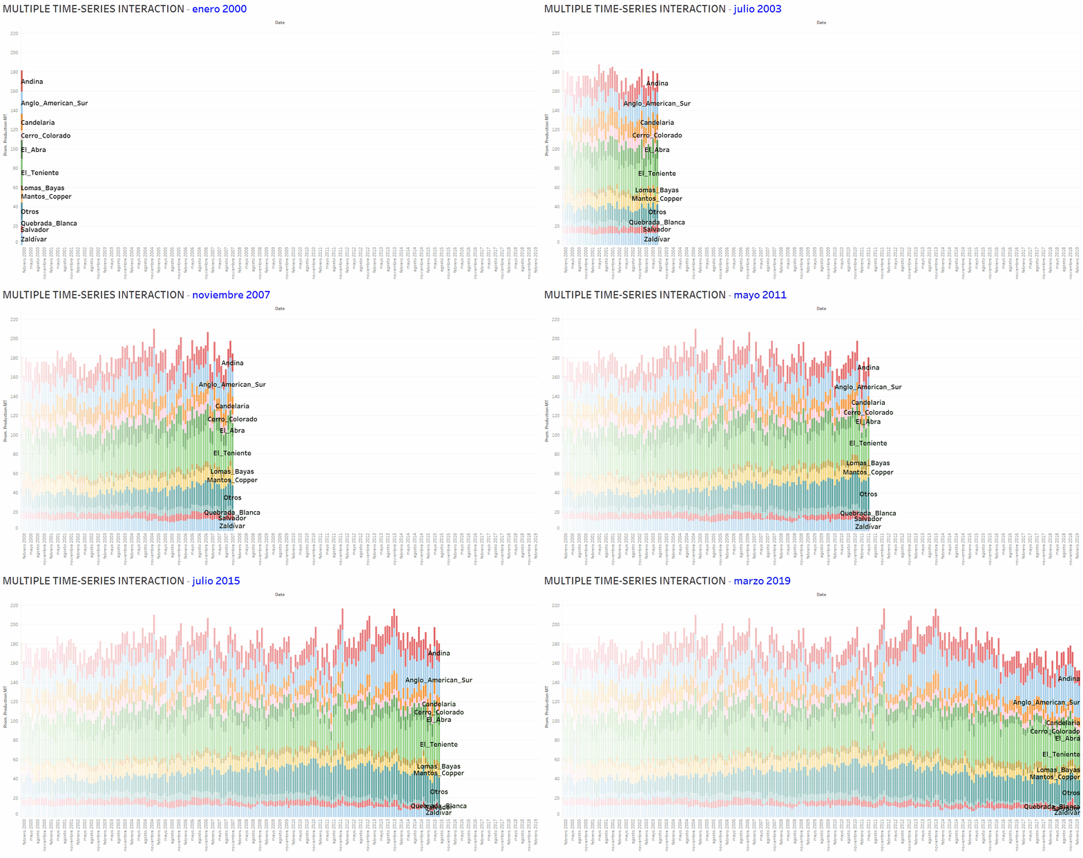
Regarding the MULTIVARIATE Machine Learning/Time Series analysis and forecasting, the basic idea is to take into account and access not only the autocorrelation of individual Time Series but also the hiding patterns encapsulated in possible interactions between the set of involved Time Series. The animation below shows the copper production time evolution (from January 2000 to March 2019) corresponding to 12 companies operating in Chile.
The objective, in a first approach to this problem, is obtaining a linear-regression-equation that could be used as a “CALCULATOR” to perform the final forecast of a target Time Series. The latest is considered the “dependent variable”; the remained Time-Series are “independent variables”. To achieve the result, a workflow available at KNIME Analytics Platform website, which includes a PARAMETER OPTIMIZATION shame, was modified and adapted for the present analytical tasks. The workflow, depicted in the figure below, uses a Linear Regression Learner (LRL) of the powerful H2O.ai Machine Learning Library (a KNIME fully INTEGRATED feature). The optimization shame addresses the tuning of the LRL hyper-parameters issue.

For the present illustrative proposes, the results are good enough: low dispersion of points in the scatter plot, and not too much difference between real and predicted curves.
The final step of the proposed MULTIVARIATE workflow will be use measured or reported values of the “independent variables” and the “CALCULATOR” to forecast the target Time Series. Another possibility, far more complex and challenging, is feed-in the “CALCULATOR” with forecasted values, obtained by applying the UNIVARIATE analysis workflow described previously. In a future post, this issue will be addressed and the full power of R-Scripting and KNIME Analytics Platform INTEGRATION will be unleashed.
Please leave your comments below, and kindly share and contact me if you require additional information.


Comments